How To Decide Which Model My Data Is In R

Model pick 101, using R

Quick and dirty markup of simple model selection using R

What're we doing?

Since this is a very introductory look at model selection nosotros assume the data you've acquired has already been cleaned, scrubbed and fix to go. Data cleaning is a whole subject in and of itself and is actually the main fourth dimension-sink of any Information Scientist. Get to the terminate of this commodity if you want to download the information for yourself and follow forth!

Edit: I've made a "sequel" to this article about visualizing and plotting the model we observe if you want to check that out after reading this one!:

Make sure to follow my contour if you lot savor this article and want to meet more!

Lets look at the pipeline:

This is the skeleton I use for creating a unproblematic LM or GLM:

Create a base-model using all available variables and data
Factorize chiselled variables if R didn't do the task
Add relevant power-transformations
Add relevant variable interaction
Remove insignificant variables with relevant testing criteria
- Echo step three–five until you've wearied your options
Remove any outlying datapoints
Evaluate your model
Visualizing your findings

i. Creating a base-model

Lets get-go by setting up a workspace and loading our information. In this case we're working on a dataset describing employment-status of women based on whether or not you're a foreigner, the amount of government-entitled support (log-transformed), age, years of instruction and the number of children (spread in ii categorical variables 'immature.children' and 'school.children'):

            rm(list=ls()) # "Clear current R environment"            setwd("C:/R/Workspace") # Setting upward your workspace
dat <- read.table("employment_data.txt", header=T) # Load that data
str(dat)
summary(dat)

which outputs:

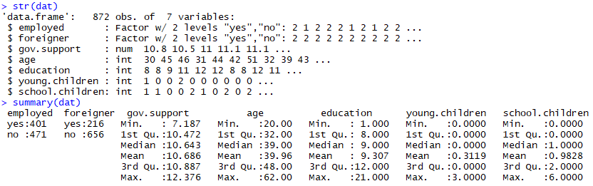
The first thing we detect is that our response-variable is binomial (apparently) suggesting that we have a binomial distribution which means nosotros'll have to fit a GLM instead of a traditional LM:

            fit.1 <- glm(employed == "yes" ~ ., information = dat, family unit = binomial)
summary(fit.1)

This fit is the most general fit we can apply past default, information technology fits a binomial model (family unit = binomial) with respect to the response-variable "employed" having a value "aye", using every variable in the dataset (~ .) giving us the post-obit output:

Right, and then a few problems right off the bat, nosotros don't like seeing p-values above 0.05, much less above 0.1, but before we recklessly remove them lets cheque for variable interactions and ability-transformations beginning!

2. Factorizing categorical variables

Lets consider the possibility that at that place's a categorical difference between not having any children and actually having any number of children larger than zero, thus we add the categorical variables for having 0 children: 'factor(young.children == 0)', 'gene(schoolhouse.children == 0)' and a combined factor for not having any children at all 'factor(immature.children + school.children == 0)'

We can update our fit with the new variables:

            tempfit <- update(fit.1, .~. + factor(young.children == 0)              
              + factor(school.children == 0)
              + factor(young.children +              
              school.children == 0))
summary(tempfit)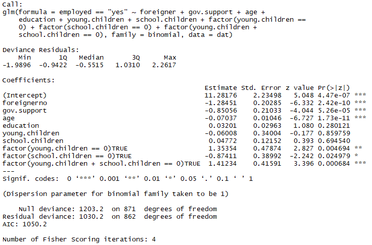

So we've already improved our model a bit in terms of AIC from 1066.eight to 1050.2! Lets accept a look at our continuous variables and watch for possible power-transformations:

3. Adding relevant power-transformations

A neat way to look for potential ability-transformations of a binomial distribution is using this custom function:

            logit.plot <- function(x, y, h, link='logit', xlab=deparse(substitute(10)), yname=deparse(substitute(y)), ylab, rug=T, data, …){
              if(!missing(information)){
              telephone call <- match.call()
              dataPos <- match("data",names(call))
              return(invisible(with(data, eval(call[-dataPos]))))
              }
              if (length(levels(factor(y)))!=2) end('y must be binary')
              succes <- levels(factor(y))[ii]
              if (missing(ylab)) ylab <- paste(binomial(link)$link,' P{',yname,'=',succes,'|',xlab,'}', sep='', collapse='')
              if (is.factor(y)) y <- every bit.numeric(y==levels(y)[two])
              x.seq <- seq(min(x),max(x),length=101)
              smooth <- binomial(link)$linkfun(ksmooth(x, y, 'normal', h, x.points=x.seq)$y)
              plot(smooth~x.seq, ylab=ylab, xlab=xlab, blazon='l',…)
              if (rug) rug(x)
              invisible(xy.coords(10 = x.seq, y = smooth, xlab = xlab, ylab = ylab))
}

It'south actually decently simple, information technology plots the link(E[y|x]) against 10 with E[y|x] estimated using a Nadaraya-Watson kernel regression estimate:

This take the following arguments:
x — Your explanatory variables
y — The binary event variable
h — Bandwidth for the Nadaraya-Watson kernel regression guess
information — Cocky explanatory
… — Whatsoever boosted arguments y'all want to pass to plot()

Using this office iterating over different bandwidths nosotros become the following kinds of plot:

            for(i in seq(2.5,10,length.out = six))
              logit.plot(x = age, y = employed == 'yes', h = i, data = dat, chief = paste0("bandwidth = ",i))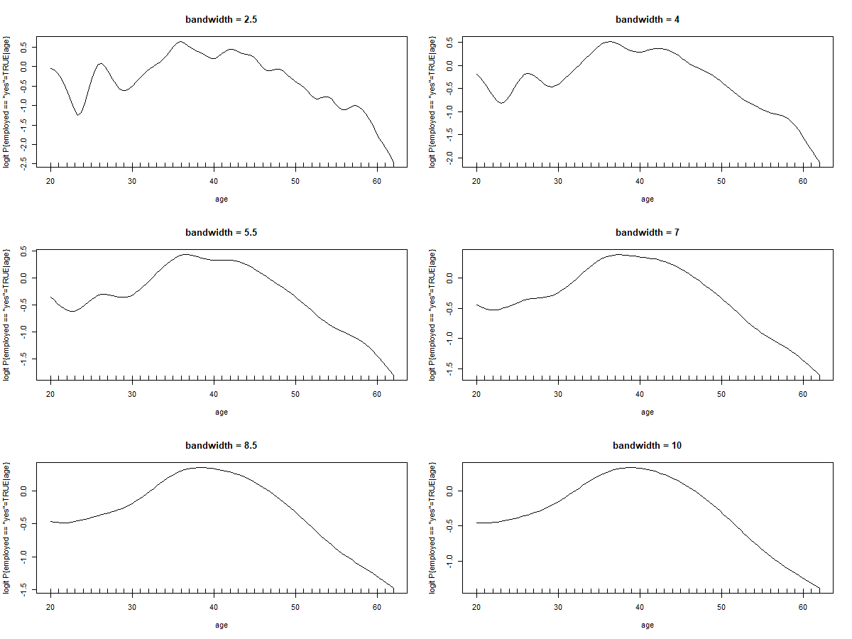

In this instance with 'historic period' we tin can run into that the role begins smoothing around a bandwidth around vii, the graph could approximate a 2. or maybe 3. degree polynomial, the same is truthful for 'teaching' and 'gov.support' but for simplicity nosotros'll consider the instance of all 3 taking shape equally 2. caste polynomials:

            tempfit <- update(tempfit, .~. + I(age^2)              
              + I(education^2)
              + I(gov.support^2))
summary(tempfit)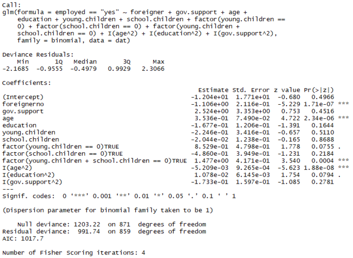

Quite the improvement in terms of AIC, from 1050.2 to 1017.7! Lots of insignificant variables though!

This is our first attempt at a "full" model, so lets define this equally our 'fit.2' and continue.

            fit.2 <- tempfit

4. Calculation variable interaction

The easiest way to check for variable interaction is using the R-function 'add1', this is simply the case of defining a scope to test and which test to utilize when testing relative to the original model. F-tests are commonly only relevant for LM and AOV models then we can 'safely' ignore that testing criteria, we'll instead exist using a χ²-examination (Chisq or Chi²):

            add1(fit.two, scope = .~. + .^two, test="Chisq")

This scope is simply asking to examination the current model (.~.) plus interaction between existing variables (+ .^2), this will output a lot of interactions, some with statistically pregnant P-values, simply it tin be annoying to manually sort through, so lets sort the list so nosotros get the lowest P-values on the top:

            add1.examination <- add1(fit.2, scope = .~. + .^2, test="Chisq")
add1.test[social club(add1.test$'Pr(>Chi)'),]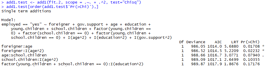

Correct, so it seems like in that location might be an interaction betwixt the greenhorn and age variables. One matter to consider before simply adding the interaction with the lowest P-value is whether or not this makes sense in context of our electric current model, right now historic period² is actually the most significant variable in our model and then nosotros might fence that adding the interaction between foreigner and age² is more intuitive, for simplicity we'll stick with the greenhorn:age interaction.

Lets test for more interactions afterwards adding the variable interaction greenhorn:age:

            add1.examination <- add1(update(fit.2, .~. + greenhorn:age), scope = .~. + .^two, examination="Chisq")
add1.test[order(add1.test$'Pr(>Chi)'),]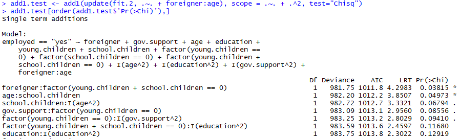

At present it seems like there'south a meaning interaction in foreigner:factor(young.children + school.children == 0)

After a few rounds of this we end upwardly seeing no new statistically meaning interactions, past the end nosotros've added the following interactions:
+ greenhorn:age
+ foreigner:factor(immature.children + school.children == 0)
+ age:school.children
+ gov.support:factor(young.children == 0)

So lets update our fit with the new variable interactions equally follows:

            fit.iii <- update(fit.ii, .~.              
+ foreigner:historic period              
+ foreigner:factor(immature.children + schoolhouse.children == 0)              
+ age:school.children              
+ gov.back up:factor(immature.children == 0))            summary(fit.3)

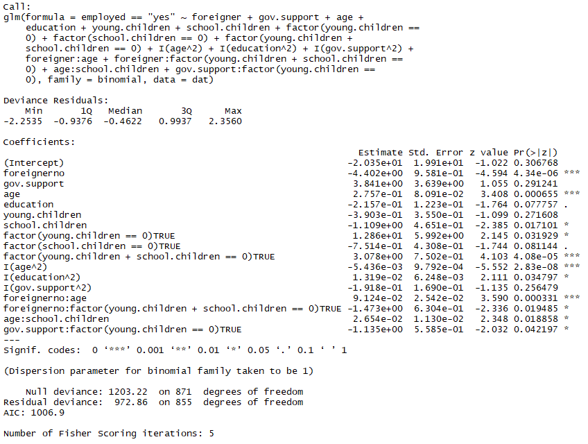
A small improvement in AIC in one case more, from 1017.vii to 1006.9.

five. Removing insignificant variables

This process is quite similar to the concluding 1 in step 4. We'll simply be using the drop1 function in R now instead of add1, and due to u.s.a. seeking to remove instead of appending variables we seek the highest P-value instead of the lowest (we'll nevertheless use χ²-test as our criteria):

            drop1.exam <- drop1(fit.iii, test="Chisq")
drop1.test[rev(guild(drop1.test$'Pr(>Chi)')),]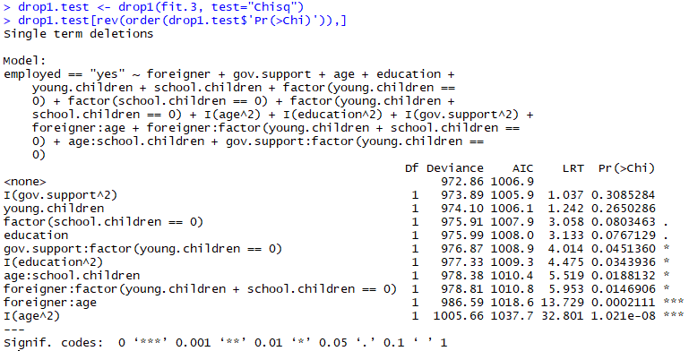

This tells u.s.a. mostly the aforementioned as our model-summary, gov.support² definitely dosn't seem to exist statistically significant, so we'll remove that start and so on then forth, we stop up removing the following variables:
- gov.support²
- young.children
- didactics
- education²

After those accept been removed nosotros run into that all the remaining variables are statistically meaning, so lets update our fit by removing the variables listed above:

            fit.4 <- update(fit.three, .~.              
— I(gov.back up^two)              
— young.children              
— education              
— I(education^two))            summary(fit.4)

Nice, some other comeback in AIC although marginal and insignificant, the main advantage of this model over our previous is the added simplicity inherent in the reduced number of explanatory variables!

1 might wonder "Why aren't nosotros removing the gov.support variable? It's conspicuously insignificant when looking at the summary of our model!" this is due to the principle of marginality which prohibits u.s. from removing an insignificant variable if said variable has a significant interaction with another, similar gov.support:factor(immature.children == 0).

You lot might fence that removing gov.back up would be beneficial to the simplicity of the model given that it's clearly insignificant and that the interaction with the young.children == 0 variable is only marginally pregnant (p = 0.435), all the same upon further inspection when removing gov.support from the model the variable-interaction splits into ii variables for True and FALSE, thus not giving us any added simplicity, the AIC, all other coefficients likewise equally the zero- and residue deviance stays the exact same and past that account I close to get out it in the model.

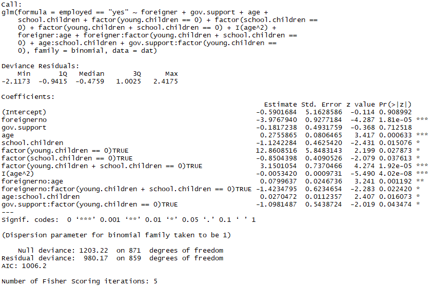
Doing an add1 and a drop1 exam on our new and improved model shows us at that place're no new interactions that are significant and that all current variables are significant so nosotros're done! The terminal fit is:

            glm(employed == "yes" ~ foreigner              
+ gov.support              
+ historic period              
+ schoolhouse.children              
+ factor(young.children == 0)              
+ factor(school.children == 0)              
+ factor(immature.children + school.children == 0)              
+ I(historic period^two)              
+ foreigner:age              
+ foreigner:cistron(immature.children + schoolhouse.children == 0)              
+ historic period:school.children              
+ gov.support:cistron(young.children == 0), family = binomial, data = dat)

half-dozen. Removing outliers

And then now that we take a model we're satisfied with we tin can look for outliers that negatively effect the model.

Using the "automobile" package https://www.rdocumentation.org/packages/car/versions/1.0-2 nosotros can use the influencePlot() and outlierTest() functions to find potential outlier:

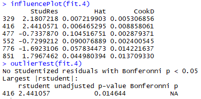
We see that the datapoint 416 is classified as an outlier in both tests, nosotros can take a wait at the point in a few of our plots to gauge whether or not to remove information technology:

            par(mfrow = c(2, 2)) # 2 row(s), two column(south)            plot(fit.4, col=ifelse(as.integer(rownames(dat))==416, "red", "blackness"), pch=20)

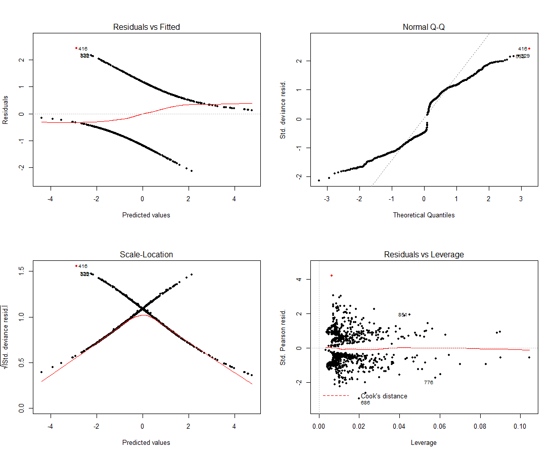
It seems similar this could very well be screwing a bit with our model, notation that we should actually be using pearson residuals to gauge our models fit so the fact that we don't have anything close to a straight line in the upper left plot is fine, Q-Q plots are irrelevant for this kind of model as well.

Lets try removing the point and have a look at the new fit:

            terminal.fit <- update(fit.4, data = dat[-c(416),])
summary(final.fit)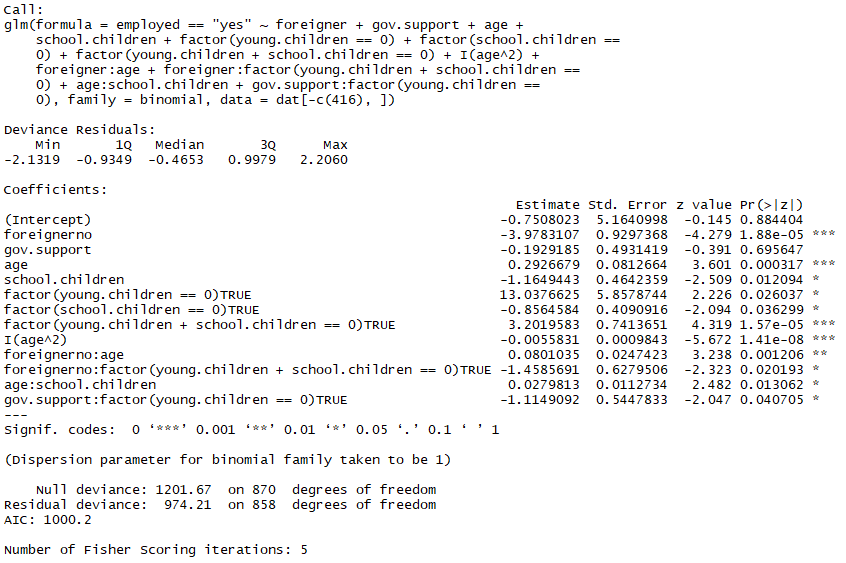

Down to almost 1000 AIC from the original 1067, this isn't really a relevant measure of operation when comparing the AIC of 2 unlike sets of data (since we removed betoken 416), we would actually have to conclude that 416 was an outlier in the initial model likewise, remove it and then compare the AIC value of the initial model without point 416 to our terminal fit without point 416 equally well.

Looking at another circular of influencePlot() and outlierTest() we detect that datapoint 329 is acting out equally well, however looking at the actual plots nosotros see that nosotros can't really justify a removal of the information like nosotros could with 416. This is our concluding fit.

vii. Model evaluation

And then now that we have a concluding fit where nosotros can't confidently add or remove any interactions variables and other transformations it's time to evaluate if our model really fits our information and if in that location's even a statistically meaning difference betwixt our final fit and the offset "naive" fit.

Lets start past taking a await at our fitted values vs. the Pearson residuals:

            par(mfrow = c(1, one)) # 2 row(s), 2 column(s)
plot(p.resid ~ fit.val)
lines(ksmooth(y = p.resid, x = fit.val, bandwidth=.ane, kernel='normal'), col='blue')
abline(h=0)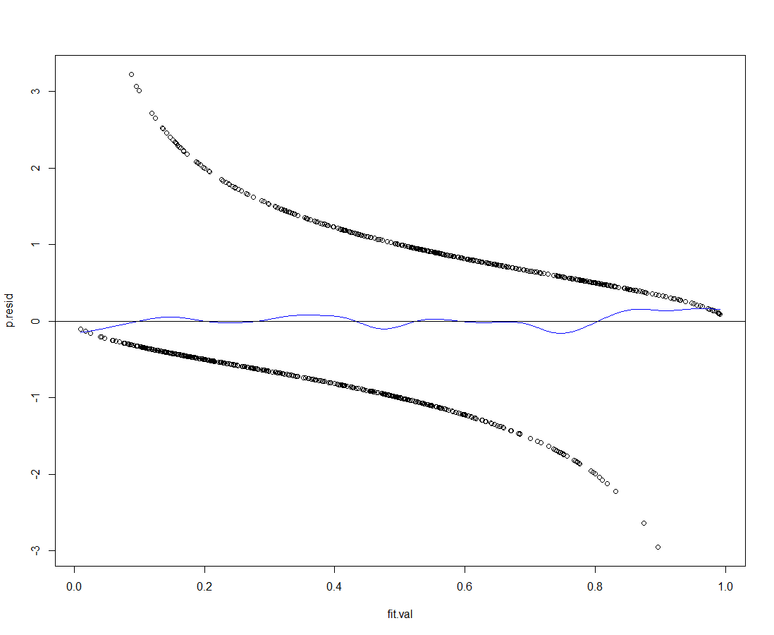

This is a pretty decent fit, lets take a look at the fit for the major explanatory variables as well:

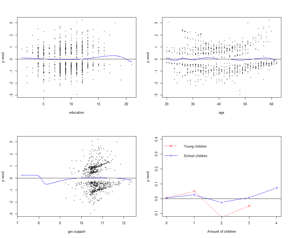
With the exception of 'gov.support' everything looks quite squeamish, also the reason for the bend in 'gov.support' seems to be a single outlier in which someone was granted a essentially lower amount of support compared to all our other points of data.

Checking for potential overfitting

Overfitting is the blight of all statistical modelling, how tin can you make sure your model isn't just fitting to the verbal data you fed it? The goal is to brand a model which generalizes and doesn't but cater to the current information at hand. Then how do we test if our model is overfitting on our data?

A popular metric to test is the delta value generated through Cross-Validation, we can calculated these by using the cv.glm function from the 'boot' package and compare our terminal fit to our first!

            cv.glm(dat[-c(416),], final.fit, K = 13)$delta
cv.glm(dat[-c(416),], update(fit.1, information = dat[-c(416),]), K = thirteen)$delta

In the code to a higher place we're using thou-fold cross-validation with g = 13 (since xiii is a factor of 871 which is the length of our data after removing the outlier) this means we're splitting our data in 13 'chunks'.

The delta values is a vector wherein the get-go component is the raw cross-validation estimate of prediction error and the second component is the adjusted cross-validation gauge (designed to recoup for the bias introduced by not using an exhaustive testing methods such every bit leave-one-out )

Running the code higher up yields the following delta-values, annotation that these are subject to some random variance and so you might not go the verbal same values:

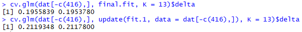
The prediction error is lower for the terminal fit, even when testing with cross-validation. Thus nosotros tin presume that our model hasn't been overfitting on our information!

The concluding slice of the puzzle

And so at present nosotros've ended that our model is actually a pretty decent fit for our data, but is information technology a statistically pregnant difference from the "naive" model without any transformations and variable interactions? We can employ an ANOVA test for this, we just have to remove the same betoken of data in both fits:

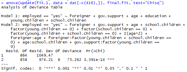
There'southward definitely a meaning deviation between the 2 fits, we can happily conclude that our hard piece of work has paid off!

viii. Model visualization

At present that we've gotten ourselves a model, how do we actually visualize and interpret what it says almost the relationships in our data?

Accept a look at the post-obit walk-trough which uses the same information and model every bit this commodity!:

Closing remarks

Please keep in heed that this is purely introductory and that this isn't an exhaustive analysis or conclusion! If we were more rigorous in our pursuit we would've incorporated Cross-Validation tests and ANOVA tests on each new iteration of our model, ie. whenever we add a new variable, interaction or power-transformation.

Feel free to message me if you lot have whatever questions and delight correct me if you lot experience like I missed something or did something wrong, practice keep in mind that this is suppose to serve as an introduction to modelling in R, I'm well aware that this process is highly simplified compared to more advanced methods!

If you want to attempt your luck with this same dataset give it a become here: https://github.com/pela15ae/statmod/blob/master/employment_data.txt

The data is Danish so to convert the headers and categorical values to English language run this piece of code:

            names(dat) <- c("employed", "greenhorn", "gov.back up", "historic period", "instruction", "young.children", "school.children")
levels(dat$employed)[1] <- "yeah"
levels(dat$employed)[2] <- "no"
levels(dat$foreigner)[i] <- "yes"
levels(dat$foreigner)[2] <- "no"