What Statistical Test To Use When Comparing Pre And Post Survey Data

Introduction

This folio shows how to perform a number of statistical tests using SPSS. Each section gives a brief description of the aim of the statistical exam, when information technology is used, an case showing the SPSS commands and SPSS (oftentimes abbreviated) output with a brief estimation of the output. You can see the page Choosing the Correct Statistical Exam for a table that shows an overview of when each test is appropriate to utilise. In deciding which examination is appropriate to apply, it is important to consider the type of variables that you lot have (i.e., whether your variables are categorical, ordinal or interval and whether they are ordinarily distributed), encounter What is the deviation between categorical, ordinal and interval variables? for more information on this.

Almost the hsb data file

Nearly of the examples in this page will use a information file called hsb2, high school and beyond. This data file contains 200 observations from a sample of high school students with demographic information about the students, such as their gender (female), socio-economic status (ses) and ethnic background (race). It also contains a number of scores on standardized tests, including tests of reading (read), writing (write), mathematics (math) and social studies (socst). Y'all can get the hsb data file by clicking on hsb2.

One sample t-examination

A i sample t-test allows us to exam whether a sample mean (of a normally distributed interval variable) significantly differs from a hypothesized value. For example, using the hsb2 data file, say we wish to test whether the average writing score (write) differs significantly from 50. Nosotros tin do this equally shown below.
                t-test  /testval = l  /variable = write.              
The mean of the variable write for this item sample of students is 52.775, which is statistically significantly different from the test value of 50. We would conclude that this group of students has a significantly college mean on the writing examination than 50.

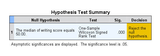
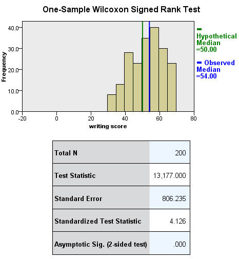
One sample median test

A i sample median examination allows united states to test whether a sample median differs significantly from a hypothesized value. We volition use the aforementioned variable, write, as we did in the one sample t-examination example above, merely nosotros practice not need to assume that it is interval and commonly distributed (we only need to assume that write is an ordinal variable).
                nptests /onesample test (write) wilcoxon(testvalue = 50).              

Image spss_whatstat_median1

Image spss_whatstat_median2

Binomial test

A one sample binomial test allows the states to test whether the proportion of successes on a two-level categorical dependent variable significantly differs from a hypothesized value. For example, using the hsb2 information file, say we wish to test whether the proportion of females (female person) differs significantly from 50%, i.e., from .5. Nosotros tin can practice this as shown beneath.
                npar tests  /binomial (.5) = female.              
The results indicate that there is no statistically meaning difference (p = .229). In other words, the proportion of females in this sample does not significantly differ from the hypothesized value of l%.

Chi-square goodness of fit

A chi-square goodness of fit test allows us to test whether the observed proportions for a categorical variable differ from hypothesized proportions. For example, let'due south suppose that nosotros believe that the general population consists of 10% Hispanic, 10% Asian, 10% African American and 70% White folks. We want to examination whether the observed proportions from our sample differ significantly from these hypothesized proportions.
                npar examination   /chisquare = race  /expected = 10 ten x 70.              
These results show that racial composition in our sample does not differ significantly from the hypothesized values that we supplied (chi-foursquare with 3 degrees of freedom = 5.029, p = .170).

2 independent samples t-test

An independent samples t-test is used when you lot want to compare the ways of a normally distributed interval dependent variable for two independent groups. For example, using the hsb2 data file, say we wish to test whether the mean for write is the same for males and females.
                t-test groups = female person(0 1)   /variables = write.              
Because the standard deviations for the ii groups are similar (10.3 and 8.1), we volition utilize the "equal variances assumed" test. The results indicate that at that place is a statistically meaning difference between the hateful writing score for males and females (t = -3.734, p = .000). In other words, females have a statistically significantly higher mean score on writing (54.99) than males (fifty.12).

Encounter also

SPSS Learning Module: An overview of statistical tests in SPSS

Wilcoxon-Isle of man-Whitney test

The Wilcoxon-Mann-Whitney examination is a non-parametric analog to the independent samples t-test and tin can exist used when you do non assume that the dependent variable is a unremarkably distributed interval variable (you only assume that the variable is at least ordinal). Y'all will observe that the SPSS syntax for the Wilcoxon-Mann-Whitney test is almost identical to that of the independent samples t-test. Nosotros will use the aforementioned information file (the hsb2 data file) and the same variables in this example equally we did in the independent t-test example to a higher place and will non assume that write, our dependent variable, is ordinarily distributed.

                npar test  /thou-w = write by female(0 1).              
                              
The results suggest that there is a statistically pregnant deviation betwixt the underlying distributions of the write scores of males and the write scores of females (z = -3.329, p = 0.001).

See too

FAQ: Why is the Mann-Whitney significant when the medians are equal?

Chi-foursquare examination

A chi-foursquare exam is used when yous want to see if there is a relationship between two categorical variables. In SPSS, the chisq option is used on the statistics subcommand of the crosstabs command to obtain the exam statistic and its associated p-value. Using the hsb2 data file, allow'southward see if at that place is a relationship betwixt the type of school attended (schtyp) and students' gender (female). Call back that the chi-square exam assumes that the expected value for each cell is v or higher. This assumption is easily met in the examples below. Still, if this assumption is non met in your information, delight see the department on Fisher's verbal exam below.
                crosstabs  /tables = schtyp by female person  /statistic = chisq.              
These results indicate that in that location is no statistically significant human relationship between the type of schoolhouse attended and gender (chi-square with one degree of freedom = 0.047, p = 0.828).

Let's wait at another example, this time looking at the linear relationship between gender (female) and socio-economic status (ses). The point of this example is that one (or both) variables may take more than ii levels, and that the variables practice not accept to accept the aforementioned number of levels. In this example, female has two levels (male and female) and ses has three levels (low, medium and high).
                crosstabs  /tables = female person by ses  /statistic = chisq.              
Again we find that there is no statistically significant human relationship between the variables (chi-square with two degrees of freedom = 4.577, p = 0.101).

See as well

SPSS Learning Module: An Overview of Statistical Tests in SPSS

Fisher'due south exact test

The Fisher'due south exact test is used when yous want to conduct a chi-foursquare exam but one or more of your cells has an expected frequency of five or less. Call back that the chi-foursquare examination assumes that each cell has an expected frequency of five or more, but the Fisher'southward exact test has no such supposition and can exist used regardless of how small the expected frequency is. In SPSS unless yous have the SPSS Exact Test Module, you lot tin can but perform a Fisher's exact test on a 2×ii tabular array, and these results are presented by default. Please see the results from the chi squared example higher up.

One-way ANOVA

A ane-mode analysis of variance (ANOVA) is used when you have a categorical independent variable (with two or more categories) and a normally distributed interval dependent variable and yous wish to test for differences in the means of the dependent variable broken down by the levels of the contained variable. For example, using the hsb2 information file, say we wish to exam whether the mean of write differs between the 3 programme types (prog). The control for this exam would be:
                oneway write by prog.              
The mean of the dependent variable differs significantly among the levels of plan type. However, we do not know if the difference is betwixt simply ii of the levels or all 3 of the levels. (The F test for the Model is the same as the F test for prog considering prog was the only variable entered into the model. If other variables had besides been entered, the F test for the Model would accept been different from prog.) To run across the mean of write for each level of plan type,
                means tables = write by prog.              
From this we can see that the students in the academic program have the highest mean writing score, while students in the vocational program take the everyman.

See also

SPSS Textbook Examples: Design and Assay, Chapter seven

SPSS Textbook Examples: Applied Regression Analysis, Chapter eight

SPSS FAQ: How tin I do ANOVA contrasts in SPSS?

SPSS Library: Understanding and Interpreting Parameter Estimates in Regression and ANOVA

Kruskal Wallis exam

The Kruskal Wallis examination is used when you accept one independent variable with two or more than levels and an ordinal dependent variable. In other words, it is the non-parametric version of ANOVA and a generalized form of the Isle of mann-Whitney exam method since information technology permits two or more groups. Nosotros volition utilize the aforementioned data file equally the one manner ANOVA example above (the hsb2 data file) and the same variables as in the example above, but we will not assume that write is a commonly distributed interval variable.
                npar tests  /k-w = write by prog (1,3).              
If some of the scores receive tied ranks, and so a correction factor is used, yielding a slightly dissimilar value of chi-squared. With or without ties, the results indicate that at that place is a statistically significant difference amid the three type of programs.

Paired t-exam

A paired (samples) t-test is used when y'all have two related observations (i.e., two observations per subject) and you lot want to encounter if the means on these two normally distributed interval variables differ from one another. For example, using the hsb2 data file nosotros will test whether the mean of read is equal to the mean of write.
                t-test pairs = read with write (paired).              
These results indicate that the mean of read is not statistically significantly different from the mean of write (t = -0.867, p = 0.387).

Wilcoxon signed rank sum test

The Wilcoxon signed rank sum test is the non-parametric version of a paired samples t-test. You employ the Wilcoxon signed rank sum examination when you practise not wish to assume that the departure between the 2 variables is interval and normally distributed (but you practise assume the difference is ordinal). Nosotros will apply the same example as to a higher place, but we will not assume that the difference between read and write is interval and normally distributed.
                npar test  /wilcoxon = write with read (paired).              
The results suggest that at that place is not a statistically significant divergence between read and write.

If you believe the differences between read and write were not ordinal but could merely exist classified as positive and negative, then you may want to consider a sign exam in lieu of sign rank test. Again, we will employ the aforementioned variables in this instance and assume that this difference is not ordinal.
                npar test  /sign = read with write (paired).              
We conclude that no statistically significant difference was found (p=.556).

McNemar examination

You would perform McNemar's test if yous were interested in the marginal frequencies of two binary outcomes. These binary outcomes may be the same consequence variable on matched pairs (like a case-control study) or two outcome variables from a single group. Continuing with the hsb2 dataset used in several in a higher place examples, let us create two binary outcomes in our dataset: himath and hiread. These outcomes can be considered in a 2-way contingency table. The aught hypothesis is that the proportion of students in the himath grouping is the same as the proportion of students in hiread grouping (i.e., that the contingency tabular array is symmetric).
                compute himath = (math>sixty). compute hiread = (read>threescore). execute.  crosstabs   /tables=himath  Past hiread   /statistic=mcnemar   /cells=count.              
McNemar'due south chi-square statistic suggests that there is not a statistically pregnant difference in the proportion of students in the himath grouping and the proportion of students in the hiread group.

Ane-way repeated measures ANOVA

You would perform a i-mode repeated measures analysis of variance if yous had 1 categorical independent variable and a normally distributed interval dependent variable that was repeated at least twice for each subject. This is the equivalent of the paired samples t-exam, but allows for two or more levels of the chiselled variable. This tests whether the hateful of the dependent variable differs by the categorical variable. We have an example data set up called rb4wide, which is used in Kirk's book Experimental Design. In this data gear up, y is the dependent variable, a is the repeated measure and south is the variable that indicates the subject area number.
                glm y1 y2 y3 y4  /wsfactor a(4).              
Y'all will detect that this output gives four different p-values. The output labeled "sphericity causeless" is the p-value (0.000) that you would get if you lot assumed compound symmetry in the variance-covariance matrix. Because that assumption is often not valid, the three other p-values offering various corrections (the Huynh-Feldt, H-F, Greenhouse-Geisser, G-G and Lower-spring). No matter which p-value you apply, our results indicate that we take a statistically significant effect of a at the .05 level.

See also

SPSS Textbook Examples from Design and Analysis: Chapter sixteen

SPSS Library: Advanced Problems in Using and Agreement SPSS MANOVA

SPSS Code Fragment: Repeated Measures ANOVA

Repeated measures logistic regression

If yous have a binary outcome measured repeatedly for each subject and you lot wish to run a logistic regression that accounts for the result of multiple measures from single subjects, you can perform a repeated measures logistic regression. In SPSS, this can be done using the GENLIN control and indicating binomial as the probability distribution and logit as the link function to be used in the model. The do data file contains 3 pulse measurements from each of 30 people assigned to 2 different diet regiments and 3 different exercise regiments. If we define a "high" pulse every bit being over 100, we tin then predict the probability of a loftier pulse using diet regiment.
                Go FILE='C:mydatahttps://stats.idre.ucla.edu/wp-content/uploads/2016/02/practice.sav'.              
                GENLIN highpulse (REFERENCE=LAST)   BY diet (society = DESCENDING) /MODEL diet    DISTRIBUTION=BINOMIAL   LINK=LOGIT /REPEATED SUBJECT=id CORRTYPE = EXCHANGEABLE.              
These results bespeak that nutrition is not statistically significant (Wald Chi-Foursquare = 1.562, p = 0.211).

Factorial ANOVA

A factorial ANOVA has two or more categorical independent variables (either with or without the interactions) and a single normally distributed interval dependent variable. For example, using the hsb2 data file we volition look at writing scores (write) as the dependent variable and gender (female) and socio-economic status (ses) as contained variables, and we will include an interaction of female by ses. Note that in SPSS, you exercise non need to have the interaction term(south) in your information fix. Rather, you can have SPSS create it/them temporarily by placing an asterisk between the variables that volition make up the interaction term(south).
                glm write past female ses.                                              
These results indicate that the overall model is statistically significant (F = 5.666, p = 0.00). The variables female and ses are also statistically significant (F = sixteen.595, p = 0.000 and F = 6.611, p = 0.002, respectively). Withal, that interaction between female and ses is not statistically meaning (F = 0.133, p = 0.875).

Run into also

SPSS Textbook Examples from Design and Analysis: Chapter x

SPSS FAQ: How can I practise tests of simple main effects in SPSS?

SPSS FAQ: How do I plot ANOVA cell ways in SPSS?

SPSS Library: An Overview of SPSS GLM

Friedman test

You perform a Friedman exam when you have ane within-subjects independent variable with two or more levels and a dependent variable that is non interval and normally distributed (just at least ordinal). Nosotros will use this exam to make up one's mind if at that place is a deviation in the reading, writing and math scores. The zero hypothesis in this test is that the distribution of the ranks of each blazon of score (i.eastward., reading, writing and math) are the same. To carry a Friedman exam, the information demand to be in a long format. SPSS handles this for you, but in other statistical packages you volition have to reshape the data before you lot can conduct this examination.
                npar tests  /friedman = read write math.              
Friedman's chi-foursquare has a value of 0.645 and a p-value of 0.724 and is not statistically significant. Hence, in that location is no show that the distributions of the iii types of scores are different.

Ordered logistic regression

Ordered logistic regression is used when the dependent variable is ordered, but not continuous. For example, using the hsb2 data file we will create an ordered variable called write3. This variable will take the values 1, 2 and 3, indicating a low, medium or high writing score. Nosotros practise not generally recommend categorizing a continuous variable in this way; nosotros are simply creating a variable to use for this example. We volition apply gender (female), reading score (read) and social studies score (socst) equally predictor variables in this model. We volition use a logit link and on the print subcommand nosotros have requested the parameter estimates, the (model) summary statistics and the test of the parallel lines assumption.
                if write ge thirty and write le 48  write3 = 1. if write ge 49 and write le 57  write3 = 2. if write ge 58 and write le 70  write3 = 3. execute.  plum write3 with female person read socst /link = logit /print = parameter summary tparallel.              
The results indicate that the overall model is statistically significant (p < .000), equally are each of the predictor variables (p < .000). There are two thresholds for this model because there are three levels of the outcome variable. We too run into that the test of the proportional odds assumption is non-pregnant (p = .563). One of the assumptions underlying ordinal logistic (and ordinal probit) regression is that the relationship betwixt each pair of effect groups is the same. In other words, ordinal logistic regression assumes that the coefficients that depict the relationship between, say, the lowest versus all higher categories of the response variable are the same as those that draw the relationship between the next lowest category and all higher categories, etc. This is called the proportional odds assumption or the parallel regression assumption. Because the human relationship between all pairs of groups is the same, in that location is only one ready of coefficients (merely one model). If this was not the case, nosotros would demand dissimilar models (such equally a generalized ordered logit model) to depict the relationship betwixt each pair of outcome groups.

See also

SPSS Data Analysis Examples: Ordered logistic regression

SPSS Annotated Output: Ordinal Logistic Regression

Factorial logistic regression

A factorial logistic regression is used when you lot take 2 or more than chiselled contained variables but a dichotomous dependent variable. For instance, using the hsb2 information file we will utilize female person as our dependent variable, because information technology is the only dichotomous variable in our data set; certainly not because it mutual exercise to utilize gender as an upshot variable. We will utilize type of program (prog) and school type (schtyp) as our predictor variables. Considering prog is a categorical variable (it has three levels), we need to create dummy codes for information technology. SPSS will do this for you by making dummy codes for all variables listed later the keyword with. SPSS volition as well create the interaction term; merely list the two variables that will make upward the interaction separated past the keyword past.
                logistic regression female with prog schtyp prog by schtyp  /contrast(prog) = indicator(ane).              
The results indicate that the overall model is not statistically significant (LR chi2 = 3.147, p = 0.677). Furthermore, none of the coefficients are statistically significant either. This shows that the overall result of prog is not significant.

Run across as well

Annotated output for logistic regression

Correlation

A correlation is useful when y'all want to see the relationship between ii (or more) normally distributed interval variables. For instance, using the hsb2 data file we can run a correlation betwixt two continuous variables, read and write.
                correlations  /variables = read write.              
                              
In the second example, nosotros will run a correlation betwixt a dichotomous variable, female person, and a continuous variable, write. Although it is assumed that the variables are interval and usually distributed, we can include dummy variables when performing correlations.
                correlations  /variables =  female write.              
                              
In the beginning instance above, nosotros see that the correlation between read and write is 0.597. By squaring the correlation so multiplying by 100, yous can make up one's mind what pct of the variability is shared. Let'southward round 0.597 to exist 0.half-dozen, which when squared would be .36, multiplied by 100 would exist 36%. Hence read shares about 36% of its variability with write. In the output for the 2nd instance, we can encounter the correlation between write and female is 0.256. Squaring this number yields .065536, significant that female shares approximately six.5% of its variability with write.

Come across also

Annotated output for correlation

SPSS Learning Module: An Overview of Statistical Tests in SPSS

SPSS FAQ: How tin I analyze my data by categories?

Missing Data in SPSS

Simple linear regression

Simple linear regression allows usa to look at the linear relationship between i usually distributed interval predictor and one unremarkably distributed interval consequence variable. For instance, using the hsb2 information file, say we wish to await at the relationship betwixt writing scores (write) and reading scores (read); in other words, predicting write from read.
                regression variables = write read  /dependent = write  /method = enter.              
We meet that the relationship between write and read is positive (.552) and based on the t-value (10.47) and p-value (0.000), nosotros would conclude this human relationship is statistically significant. Hence, we would say there is a statistically significant positive linear relationship between reading and writing.

Encounter also

Regression With SPSS: Affiliate 1 – Simple and Multiple Regression

Annotated output for regression

SPSS Textbook Examples: Introduction to the Practice of Statistics, Affiliate x

SPSS Textbook Examples: Regression with Graphics, Chapter ii

SPSS Textbook Examples: Applied Regression Analysis, Chapter 5

Non-parametric correlation

A Spearman correlation is used when one or both of the variables are not assumed to be normally distributed and interval (but are assumed to be ordinal). The values of the variables are converted in ranks then correlated. In our example, we will look for a relationship between read and write. We will non assume that both of these variables are normal and interval.
                nonpar corr  /variables = read write  /print = spearman.              
                              
The results suggest that the relationship between read and write (rho = 0.617, p = 0.000) is statistically pregnant.

Simple logistic regression

Logistic regression assumes that the issue variable is binary (i.e., coded as 0 and 1). We have simply one variable in the hsb2 information file that is coded 0 and 1, and that is female. We understand that female is a silly outcome variable (it would brand more than sense to use it equally a predictor variable), only nosotros tin use female person equally the issue variable to illustrate how the code for this command is structured and how to interpret the output. The get-go variable listed after the logistic control is the issue (or dependent) variable, and all of the rest of the variables are predictor (or independent) variables. In our example, female volition be the outcome variable, and read volition be the predictor variable. As with OLS regression, the predictor variables must exist either dichotomous or continuous; they cannot be categorical.
                logistic regression female person with read.              
The results indicate that reading score (read) is not a statistically significant predictor of gender (i.due east., beingness female person), Wald = .562, p = 0.453. Likewise, the test of the overall model is not statistically significant, LR chi-squared – 0.56, p = 0.453.

See besides

Annotated output for logistic regression

SPSS Library: What kind of contrasts are these?

Multiple regression

Multiple regression is very like to unproblematic regression, except that in multiple regression y'all have more than one predictor variable in the equation. For case, using the hsb2 data file we will predict writing score from gender (female), reading, math, science and social studies (socst) scores.
                regression variable = write female read math science socst  /dependent = write  /method = enter.              
The results betoken that the overall model is statistically significant (F = 58.60, p = 0.000). Furthermore, all of the predictor variables are statistically significant except for read.

Encounter also

Regression with SPSS: Affiliate 1 – Unproblematic and Multiple Regression

Annotated output for regression

SPSS Frequently Asked Questions

SPSS Textbook Examples: Regression with Graphics, Chapter three

SPSS Textbook Examples: Practical Regression Assay

Analysis of covariance

Analysis of covariance is like ANOVA, except in improver to the categorical predictors you also have continuous predictors too. For example, the i mode ANOVA instance used write equally the dependent variable and prog as the contained variable. Let's add read as a continuous variable to this model, as shown below.
                glm write with read by prog.              
The results point that even after adjusting for reading score (read), writing scores still significantly differ past plan type (prog), F = 5.867, p = 0.003.

See also

SPSS Textbook Examples from Design and Analysis: Affiliate 14

SPSS Library: An Overview of SPSS GLM

SPSS Library: How do I handle interactions of continuous and categorical variables?

Multiple logistic regression

Multiple logistic regression is like uncomplicated logistic regression, except that in that location are 2 or more predictors. The predictors tin can be interval variables or dummy variables, but cannot be chiselled variables. If yous take categorical predictors, they should be coded into i or more dummy variables. Nosotros have only one variable in our data set that is coded 0 and 1, and that is female person. We understand that female is a silly outcome variable (it would make more sense to use information technology as a predictor variable), but we tin can use female as the outcome variable to illustrate how the lawmaking for this command is structured and how to interpret the output. The first variable listed after the logistic regression control is the outcome (or dependent) variable, and all of the rest of the variables are predictor (or contained) variables (listed after the keyword with). In our example, female volition be the outcome variable, and read and write volition exist the predictor variables.
                logistic regression female person with read write.              
These results show that both read and write are significant predictors of female.

See also

Annotated output for logistic regression

SPSS Textbook Examples: Applied Logistic Regression, Affiliate ii

SPSS Code Fragments: Graphing Results in Logistic Regression

Discriminant assay

Discriminant analysis is used when yous accept one or more usually distributed interval independent variables and a categorical dependent variable. It is a multivariate technique that considers the latent dimensions in the contained variables for predicting grouping membership in the categorical dependent variable. For example, using the hsb2 data file, say we wish to use read, write and math scores to predict the blazon of program a pupil belongs to (prog).
                discriminate groups = prog(1, 3)  /variables = read write math.              
Clearly, the SPSS output for this procedure is quite lengthy, and it is across the scope of this page to explain all of it. Nevertheless, the primary point is that two canonical variables are identified past the analysis, the offset of which seems to be more related to program blazon than the second.

See also

discriminant role analysis

SPSS Library: A History of SPSS Statistical Features

One-way MANOVA

MANOVA (multivariate analysis of variance) is like ANOVA, except that in that location are two or more dependent variables. In a one-way MANOVA, at that place is ane categorical independent variable and two or more than dependent variables. For example, using the hsb2 data file, say we wish to examine the differences in read, write and math broken down by programme type (prog).
                glm read write math by prog.              
The students in the dissimilar programs differ in their articulation distribution of read, write and math.

Come across also

SPSS Library: Avant-garde Issues in Using and Understanding SPSS MANOVA

GLM: MANOVA and MANCOVA

SPSS Library: MANOVA and GLM

Multivariate multiple regression

Multivariate multiple regression is used when you have 2 or more than dependent variables that are to be predicted from two or more independent variables. In our instance using the hsb2 data file, we will predict write and read from female person, math, scientific discipline and social studies (socst) scores.
                glm write read with female person math science socst.              
These results prove that all of the variables in the model take a statistically significant human relationship with the joint distribution of write and read.

Canonical correlation

Approved correlation is a multivariate technique used to examine the relationship between two groups of variables. For each prepare of variables, it creates latent variables and looks at the relationships amid the latent variables. It assumes that all variables in the model are interval and normally distributed. SPSS requires that each of the two groups of variables exist separated by the keyword with. In that location need not be an equal number of variables in the two groups (earlier and after the with).

                manova read write with math science  /discrim.                * * * * * * A n a l y due south i s   o f   V a r i a north c e -- design   1 * * * * * *   Event .. Inside CELLS Regression  Multivariate Tests of Significance (S = ii, G = -1/2, N = 97 )   Test Proper name         Value  Approx. F Hypoth. DF   Mistake DF  Sig. of F   Pillais          .59783   41.99694       4.00     394.00       .000  Hotellings      1.48369   72.32964       iv.00     390.00       .000  Wilks            .40249   56.47060       iv.00     392.00       .000  Roys             .59728  Note.. F statistic for WILKS' Lambda is exact.   - - - - - - - - - - - - - - - - - - - - - - - - - - - - - - - - - - - - -  EFFECT .. WITHIN CELLS Regression (Cont.)  Univariate F-tests with (2,197) D. F.   Variable    Sq. Mul. R  Adj. R-sq.  Hypoth. MS    Error MS           F   READ            .51356      .50862  5371.66966    51.65523   103.99081  WRITE           .43565      .42992  3894.42594    51.21839    76.03569   Variable     Sig. of F   READ              .000  WRITE             .000   - - - - - - - - - - - - - - - - - - - - - - - - - - - - - - - - - - - - -  Raw canonical coefficients for DEPENDENT variables            Function No.   Variable            one   READ             .063  WRITE            .049   - - - - - - - - - - - - - - - - - - - - - - - - - - - - - - - - - - - - -  Standardized canonical coefficients for DEPENDENT variables            Function No.   Variable            1   READ             .649  WRITE            .467  * * * * * * A due north a l y s i s   o f   V a r i a n c eastward -- design   1 * * * * * *   Correlations between DEPENDENT and canonical variables            Role No.   Variable            1   READ             .927  WRITE            .854   - - - - - - - - - - - - - - - - - - - - - - - - - - - - - - - - - - - - -  Variance in dependent variables explained by canonical variables   CAN. VAR.  Pct Var DE Cum Pct DE Pct Var CO Cum Pct CO          1       79.441     79.441     47.449     47.449   - - - - - - - - - - - - - - - - - - - - - - - - - - - - - - - - - - - - -  Raw canonical coefficients for COVARIATES            Function No.   COVARIATE           i   MATH             .067  SCIENCE          .048   - - - - - - - - - - - - - - - - - - - - - - - - - - - - - - - - - - - - -  Standardized canonical coefficients for COVARIATES            CAN. VAR.   COVARIATE           1   MATH             .628  SCIENCE          .478   - - - - - - - - - - - - - - - - - - - - - - - - - - - - - - - - - - - - -  Correlations betwixt COVARIATES and canonical variables            CAN. VAR.   Covariate           1   MATH             .929  SCIENCE          .873  * * * * * * A n a 50 y s i southward   o f   V a r i a n c e -- design   1 * * * * * *   Variance in covariates explained by canonical variables   Tin. VAR.  Pct Var DE Cum Pct DE Pct Var CO Cum Pct CO          ane       48.544     48.544     81.275     81.275   - - - - - - - - - - - - - - - - - - - - - - - - - - - - - - - - - - - - -  Regression analysis for Within CELLS mistake term  --- Individual Univariate .9500 confidence intervals  Dependent variable .. READ              reading score   COVARIATE            B        Beta   Std. Err.     t-Value   Sig. of t   MATH            .48129      .43977        .070       half dozen.868        .000  Scientific discipline         .36532      .35278        .066       5.509        .000   COVARIATE   Lower -95%  CL- Upper   MATH              .343        .619  SCIENCE           .235        .496  Dependent variable .. WRITE             writing score   COVARIATE            B        Beta   Std. Err.     t-Value   Sig. of t   MATH            .43290      .42787        .070       6.203        .000  Scientific discipline         .28775      .30057        .066       4.358        .000   COVARIATE   Lower -95%  CL- Upper   MATH              .295        .571  Scientific discipline           .158        .418   - - - - - - - - - - - - - - - - - - - - - - - - - - - - - - - - - - - - -  * * * * * * A north a fifty y s i s   o f   5 a r i a northward c e -- design   1 * * * * * *   Result .. Constant  Multivariate Tests of Significance (S = 1, G = 0, Due north = 97 )   Test Name         Value    Verbal F Hypoth. DF   Fault DF  Sig. of F   Pillais          .11544   12.78959       2.00     196.00       .000  Hotellings       .13051   12.78959       ii.00     196.00       .000  Wilks            .88456   12.78959       2.00     196.00       .000  Roys             .11544  Notation.. F statistics are exact.   - - - - - - - - - - - - - - - - - - - - - - - - - - - - - - - - - - - - -  Upshot .. CONSTANT (Cont.)  Univariate F-tests with (ane,197) D. F.   Variable   Hypoth. SS   Fault SS Hypoth. MS   Error MS          F  Sig. of F   READ        336.96220 10176.0807  336.96220   51.65523    half-dozen.52329       .011  WRITE      1209.88188 10090.0231 1209.88188   51.21839   23.62202       .000   - - - - - - - - - - - - - - - - - - - - - - - - - - - - - - - - - - - - -  EFFECT .. CONSTANT (Cont.)  Raw discriminant function coefficients            Function No.   Variable            i   READ             .041  WRITE            .124   - - - - - - - - - - - - - - - - - - - - - - - - - - - - - - - - - - - - -  Standardized discriminant function coefficients            Function No.   Variable            1   READ             .293  WRITE            .889   - - - - - - - - - - - - - - - - - - - - - - - - - - - - - - - - - - - - -  Estimates of effects for canonical variables            Canonical Variable    Parameter          i          1        2.196  * * * * * * A n a fifty y s i s   o f   V a r i a n c e -- pattern   1 * * * * * *   EFFECT .. Abiding (Cont.)  Correlations between DEPENDENT and canonical variables            Canonical Variable   Variable            1   READ             .504  WRITE            .959   - - - - - - - - - - - - - - - - - - - - - - - - - - - - - - - - - - - - -

The output above shows the linear combinations respective to the get-go canonical correlation. At the bottom of the output are the 2 approved correlations. These results point that the offset canonical correlation is .7728. The F-test in this output tests the hypothesis that the showtime approved correlation is equal to zero. Clearly, F = 56.4706 is statistically meaning. However, the second canonical correlation of .0235 is not statistically significantly different from zero (F = 0.1087, p = 0.7420).

Factor analysis

Factor assay is a form of exploratory multivariate assay that is used to either reduce the number of variables in a model or to detect relationships among variables. All variables involved in the factor analysis need to be interval and are assumed to be normally distributed. The goal of the assay is to endeavour to identify factors which underlie the variables. There may be fewer factors than variables, just there may not be more factors than variables. For our example using the hsb2 data file, let's suppose that we think that there are some common factors underlying the diverse test scores. We will include subcommands for varimax rotation and a plot of the eigenvalues. We volition use a principal components extraction and will retain two factors. (Using these options volition make our results compatible with those from SAS and Stata and are non necessarily the options that you will want to use.)
                factor   /variables read write math science socst     /criteria factors(two)    /extraction pc   /rotation varimax   /plot eigen.              
Communality (which is the contrary of uniqueness) is the proportion of variance of the variable (i.due east., read) that is accounted for past all of the factors taken together, and a very low communality can indicate that a variable may not belong with whatever of the factors. The scree plot may exist useful in determining how many factors to retain. From the component matrix table, we can come across that all 5 of the examination scores load onto the first factor, while all five tend to load not and so heavily on the 2d factor. The purpose of rotating the factors is to get the variables to load either very high or very depression on each factor. In this example, considering all of the variables loaded onto factor 1 and non on factor ii, the rotation did non aid in the estimation. Instead, it fabricated the results even more difficult to interpret.

See also

SPSS FAQ: What does Cronbach's alpha hateful?